Mastering Python in BA: Data Mining Techniques in Business Analytics

Reading Time: 9 minutes

Introduction

When it comes to Business Analytics, Data Mining plays a crucial role in helping businesses and organizations understand past and present events. It can even assist businesses in predicting and understanding future events based on historical data. These types of analytics are often referred to as descriptive, diagnostic, predictive, or prescriptive analytics. Data mining can provide useful results that can be used for decision-making within a (data-driven) business. 

This article will explore a handful of data mining techniques and how you can experiment with them using Python and some of its libraries. 

SEMMA

Let’s start by looking at the process of creating a model.

SAS Institute, a multinational developer of analytics and artificial intelligence software, created a methodology called SEMMA which helps decide what model to build and how to build it (SAS Help Center, n.d.):

1. Sample: In the first step, a representative sample of data is selected from the available dataset. The sample should be large enough to be statistically significant but small enough to be manageable for analysis. Sampling helps in reducing computational complexity and ensures that the analysis is based on a representative portion of the data.
2. Explore: In the exploration phase, the selected dataset is thoroughly examined to gain insights into its characteristics and identify potential patterns or relationships. Descriptive statistics, data visualization techniques, and exploratory data analysis (EDA) are used to understand the distributions, correlations, outliers, and other important data properties.
3. Modify: In this step, data preprocessing and feature engineering techniques are applied to prepare the data for modeling. This may involve handling missing values, dealing with outliers, transforming variables, encoding categorical variables, and creating new features. The goal is to clean and transform the data in a way that enhances the performance of predictive models.
4. Model: The modeling step involves building predictive models using various techniques such as regression, classification, clustering, or association analysis, depending on the nature of the problem and the objectives of the analysis. Multiple models may be trained and evaluated to identify the most effective approach for making predictions or uncovering patterns in the data.
5. Assess: In the final step, the performance of the models is evaluated using appropriate metrics and validation techniques. This involves assessing the models’ accuracy, robustness, and generalization ability on unseen data. Model performance may be compared against baseline models or business objectives to determine if the predictive models meet the desired criteria.

In step 4, before building the model, it is important to decide what type of model should be built. SAS mentions several analytical tools/techniques but for this article, we will focus on six techniques that fall into three different categories:

1. Classification and Prediction:
   • Linear regression
   • Decision trees
   • k-Nearest neighbors
   • Naïve Bayes
2. Association:
   • Association rules
3. Clustering:
   • k-Means

Linear regression

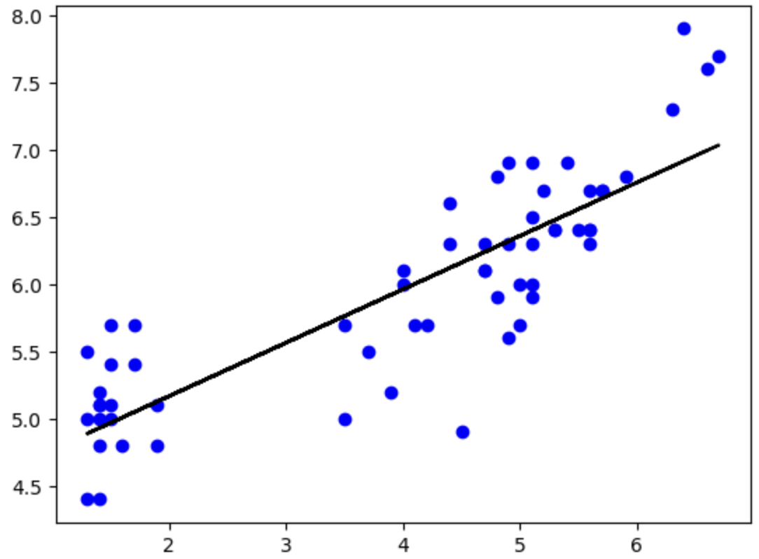
One of the most well-known techniques to perform predictions is through linear regression. Whether this is through a single linear regression model or a multiple linear regression model, the difference is whether you have/use one or multiple independent variables (X) to predict a certain outcome (Y). When using this model, there’s always a chance that the prediction (Ŷ) differs from the observation (Y). This would be referred to as an error (e) and the total collection of all these errors would be referred to as the sum of errors.

How to do this with Python:

# Start by importing the packages from Python's diverse set of libraries (in case not present, install with pip)

from pathlib import Path
import pandas as pd
from sklearn.model_selection import train_test_split
from sklearn.linear_model import LinearRegression

# Load the data from your csv file into a variable called df_file (easier to use repetitively)

df_file = pd.read_csv(r"path_to_file.csv")

# Define the independent variable from your file and put it into the variable 'X'

X = df_file[['X1']]

# Define the dependent variable and link it to a variable called y

y = df_file['Y'].values

# This important step lets you split the dataset into 4 sets for your model, 2 sets for training and two sets for testing the model. You define the relative size of the training or testing set by setting the size between 0 and 1

X_train, X_test, y_train, y_test = train_test_split(X, y, test_size=0.6,random_state=101)

# We assign the linear regression function to a variable and train this model using .fit() where we provide the training data

model_lr = LinearRegression()
model_lr.fit(X_train.values, y_train) 

# Finally we decide what we want to do with this model, we can either ask it to test the trained model with values from the csv file, or provide these values ourselves and predict its mean

predictions = model_lr.predict([[4.6]])
print(predictions.mean())


# We can even ask Python to provide details about our model or to visualize our data, in this case you may need to import additional packages

print('The shape of the dataframe is: ', df_file.shape)
print('The shape of X is: ', X.shape)
print('The shape of y is: ', y.shape)
print('The amount of NaN or Missing values in the dataframe is: ')
print(df_file.isnull().sum())

# In order to visualize we use:

import matplotlib.pyplot as plt
plt.scatter(X,y)
plt.scatter(X_train, y_train, color='b')
plt.plot(X_train, model_lr.predict(X_train.values), color='k')

Decision trees

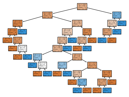
Decision trees are a simple yet powerful technique used for classification and regression tasks. They offer transparency in decision-making, making them easy to interpret for stakeholders. Decision trees can handle both numerical and categorical. They are also quite flexible and scalable as a model. However, they are susceptible to overfitting, especially when the tree becomes too deep and complex.

Using Decision trees in Python can be done as follows:

# First, make sure that you have imported and installed the necessary packages

from pathlib import Path
import pandas as pd
import seaborn as sns
import sklearn.metrics as pm
import numpy as np
import seaborn as sn
import matplotlib.pyplot as plt
from sklearn.tree import DecisionTreeClassifier
from sklearn.model_selection import train_test_split
from sklearn import svm, datasets
from sklearn import tree

# Read and load the file with data into a variable using pandas

df_file = pd.read_csv(r'path_to_file.csv')

# Define the independent variables and the dependent variable

predictors = ['X1', 'X2', 'X3']
X = pd.get_dummies(df_file[predictors])
y = df_file['Y'].values

# Just like with Linear regression, we can split the data into four sets and define the relatative size of the testing dataset and the training dataset

X_train, X_test, y_train, y_test = train_test_split(X, y, test_size=0.9, random_state=101)

# Next, we use the DecisionTreeClassifier() function to train the model using the fit() function

trained_tree = DecisionTreeClassifier()
trained_tree.fit(X_train, y_train)

# Once the model is trained, we can draw the corresponding Decision tree

drawn_tree = tree.plot_tree(fullClassTree, filled = True)
plt.figure(figsize=(50,50))

# If we wish to obtain more data about the model like its precision, we can use functions of sklearn.metrics to show this

y_pred = trained_tree(X_test)
print("The following performance scores are gathered from the training data set:")
print(f"The precision score is: ", pm.precision_score(y_test,y_pred,average=None))
print(f"The recall score is: ", pm.recall_score(y_test,y_pred,average=None))
print(f"The f-measure is: ", pm.f1_score(y_test, y_pred, average=None))

k-Nearest neighbors

K-nearest neighbors (KNN) is a simple and intuitive machine learning algorithm used for classification and regression tasks. It predicts the label or value of a new data point based on the similarity/ closeness between records. In data mining, KNN is used for classification, regression, and anomaly detection tasks in diverse fields such as text categorization, image recognition, and fraud detection.

We can also work with this technique using Python libraries:

# As before, it is important to import the necessary libraries

from pathlib import Path
import pandas as pd
from sklearn.model_selection import train_test_split
from sklearn.neighbors import KNeighborsClassifier
import matplotlib.pylab as plt

# We load the data from the csv file to a variable and define the independent and dependent variables

df_file = pd.read_csv(r'path_to_file.csv')
X = df_file.drop('Y',axis=1).values 
y = df_file['Y'].values 

# Again, we split the dataset into 4 parts and define the size of the traing set and testing set

X_train,X_test,y_train,y_test=train_test_split(X,y,test_size=0.2,random_state=101)

# For k-Nearest neigbors we use the KneighborsClassifier function to set the amount of neighbors and train the model using fit(). Note that it is key to pick the right k-value to minimize the error rates and maximize the classification performance. A good way to find this, is by running the model multiple times with different k-values and pick the one with the highest F1-measures (closest to 1 for both the Recall and the Precision)

knn_model = KNeighborsClassifier(n_neighbors=4)
knn_model.fit(X_train,y_train)

y_pred = knn_model.predict(X_test)

print(f"The f-measure is: ", pm.f1_score(y_test, y_pred, average=None))

# Or if you want to predict a specific outcome (don't use this when finding the f-measure)

y_pred = knn_model.predict([[6.5,3,5.5,1.8]])

print(y_pred)

Naïve Bayes

Naïve Bayes is a fundamental classification technique in data mining. Despite its simplicity, it’s widely used in tasks like text classification, and spam filtering. A trained Naïve Bayes model looks at the dependent variable with the highest probability when deciding what prediction to return. A Naïve Bayes trained model requires a very large number of records to obtain reliable results.

In Python, we can also use Naïve Bayes:

from sklearn.naive_bayes import MultinomialNB
from sklearn.naive_bayes import GaussianNB
import matplotlib.pylab as plt 
from sklearn.metrics import roc_curve

# There are multiple types of Naïve Bayes we choose from, in this example we use Multinomial Naïve Bayes and Gaussian Naïve Bayes. The biggest difference between them being that MultinomialNB takes the average value into account of each feature of each class, whilce GaussianNB stores the average values as well as the standard deviation of each feature for each class.

df_file = pd.read_csv(r'path_to_file.csv')
X = df_file.drop('y',axis=1).values
y = df_file['y'].values
X_train, X_test, y_train, y_test = train_test_split(X, y, test_size=0.4, random_state=101)

# For the MultinomialNB:

mnb = MultinomialNB()
mnb.fit(X_train, y_train)

y_pred = mnb.predict(X_test)
fpr_mnb, tpr_mnb, thresholds_mnb = roc_curve(y_test, y_pred)
plt.plot([0,1],[0,1],'k--')
plt.plot(fpr_mnb, tpr_mnb, label='MultinomialNB')

# For the GaussianNB:

model_GaussianNB = GaussianNB()
model_GaussianNB.fit(X_train,y_train)

y_pred = model_GaussianNB.predict(X_test)
fpr_gnb, tpr_gnb, thresholds_gnb = roc_curve(y_test, y_pred)
plt.plot([0,1],[0,1],'k--')
plt.plot(fpr_gnb, tpr_gnb, label='GaussianNB')

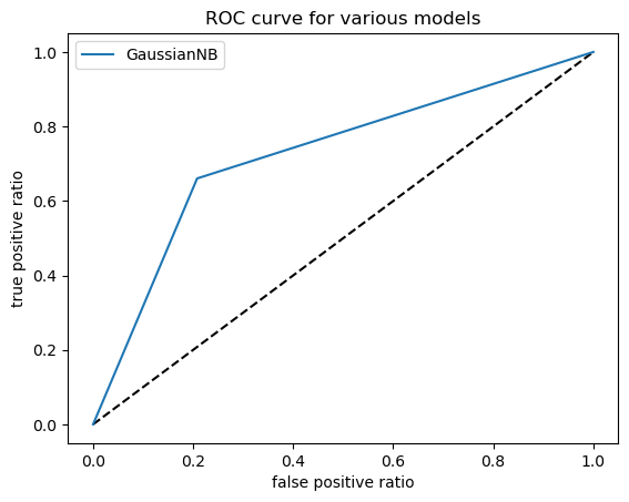
# Having picked one of the Naïve Bayes models, we can now draw an ROC (Receiver Operating Characteristic) curve to illustrate the performance of the classifier model and plot the true positive rate against the false positive rate

plt.xlabel('False positive ratio')
plt.ylabel('True positive ratio') 
plt.title('ROC curve for various models')
plt.legend()
plt.show()

# If we wish to know the AUC (Area Under the Curve) score, we can simple type the follwoing:

print("ROC AUC score:", pm.roc_auc_score(y_test, y_pred))

Association rules

Association rules is a model that is great at identifying item clusters in event-based or transaction-based databases. It is often used in retail for learning about items that are often bought together. Think about Amazon or Bol.com, whenever you are looking for an item they often suggest items to you that are based on articles that are frequently bought together with the item you’re looking at.

In Python, we can also train such models and find associations:

# For this model, it is important we have installed and imported the mlxtend library

import pandas as pd
import numpy as np
from mlxtend.preprocessing import TransactionEncoder
import matplotlib.pyplot as plt
from mlxtend.frequent_patterns import apriori
from mlxtend.frequent_patterns import association_rules

df_file = pd.read_csv(r'path_to_file.csv')

# We fill an array called transactions by using a nested for loop. This loop picks any values that hold a value other than 'nan' which has no meaning and therefore cannot be used. 

transactions = []
for i in range(len(df_file)):
    row=[]
    for j in range(len(df_file.columns)):
        if str(df_file.values[i,j])!='nan':
            row.append(str(df_file.values[i,j]))
    transactions.append(row)

# We use the TransactionEncoder() function and assign it to a variable called encoder. We then train the model using the array we created earlier.

encoder = TransactionEncoder()
trans_trained = encoder.fit(transactions).transform(transactions)

# We can retrieve the frequent itemsets which have a support higher than 0.01. Support is an estimated probability that a transaction (which is selected randonly from the database) will contain all items in the antecedent and the concequent.

df = pd.DataFrame(trans_trained, columns=encoder.columns_)
frequent_itemsets = apriori(df, min_support=0.01, use_colnames=True)

# We can also set different measures to ensure the strength of the association, such as confidence or lift ratio.

rules=association_rules(frequent_itemsets,metric="confidence",min_threshold=0.15)

rules = association_rules(frequent_itemsets, metric="lift", min_threshold=3)

# Finally we can print the frequent_itemsets

frequent_itemsets

k-Means

K-means clustering is a form of unsupervised learning and is a vital tool in Business Analytics, where data is grouped into clusters to reveal patterns. It helps in things such as customer segmentation for targeted marketing and anomaly detection for fraud prevention. This empowers businesses to make informed decisions and stay competitive.

To get an idea of how this works with Python, observe the following code:

import pandas as pd
from sklearn.cluster import KMeans
import matplotlib.pyplot as plt

# We must first load the data from our csv file

df_file = pd.read_csv(r'path_to_file.csv')

# We then define the two columns we want to use for clustering

X = data[['Feature 1', 'Feature 2']]

# We specify the number of clusters (k) we want

k = 3

# Initialize and train the k-means model

kmeans = KMeans(n_clusters=k)
kmeans.fit(X)

# For readability we add cluster labels to the dataframe

data['cluster'] = kmeans.labels_

# Finally, we can visualize the clusters

plt.scatter(data['Feature 1'], data['Feature 2'], c=data['cluster'], cmap='viridis')
plt.scatter(kmeans.cluster_centers_[:, 0], kmeans.cluster_centers_[:, 1], s=300, c='red', marker='*', label='Centroids')
plt.xlabel('Feature 1')
plt.ylabel('Feature 2')
plt.title('K-means Clustering')
plt.legend()
plt.show()

Conclusion and tips

In conclusion, mastering data mining techniques with Python is a powerful asset for developing valuable insights. When doing so, keep consider the following:

1. Data Splitting: Ensure a balanced split between training and testing data to avoid overfitting or underfitting.
2. Technique Selection: Choose the right data mining technique tailored to the specific problem at hand.
3. Data Quality: Reliable data is paramount. Collect and verify data meticulously to ensure accuracy.
4. Data Preprocessing: Clean and standardize data to enhance model performance and interpretability.
5. Model Adjustment: Continuously refine models based on metrics like the F1 measure to optimize predictive accuracy.

By adhering to these principles and using Python’s available libraries, such as scikit-learn, you can unlock many capabilities of data mining to drive informed decision-making and achieve business objectives effectively.

Literature

Lectures and lab exercises provided during Business Intelligence & Business Analytics classes taught by Dr. Emiel Caron and Dr. Ekaterini Ioannou
SAS Help Center. (n.d.). https://documentation.sas.com/doc/en/emref/14.3/n061bzurmej4j3n1jnj8bbjjm1a2.htm